Prey population growth constrained by predators (Lotka-Volterra)

What if a growing population gets eaten by another population?

In a previous post I showed why we might expect a population to grow exponentially when not resource limited. We then extended this to the case where a population reaches some carrying capacity (using a simple and non-mechanistic logistic function).

But population growth can also be curtailed through interactions with another species population, such as a predator. In my area of study, we deal with a lot of herbivorous pests of agricultural systems. Despite the predominance of pesticides as a pest management strategy, there is a growing appreciation that "beneficial" arthropods, such as predators, will suppress pests.

Lotka-Volterra

Most ecologists will have heard the conjugation of Lotka-Volterra in reference to predator-prey dynamics, and here we will have a look at the equations that have become synonymous with their names.

To introduce another population, we require another variable to keep track of it's state (another state variable). Let's go with for predator numbers. If our unconstrained prey population growth rate can be described as where is the difference between per capita reproduction and mortality rates, it is reasonable to suppose that a predator population will have an negative effect on as a consequence of the amount of prey ingested per time. The ingestion rate per predator might depend linearly on the number of prey available or where is a predator's consumption rate of prey per available prey. Multiplying this by the total predators is the total prey consumed per time and prey population growth can be described as:

As with the prey, the predator population growth , will be proportional to the reproduction rate minus mortality. Per capita predator reproduction can be assumed to depend on the amount of prey ingested multiplied by some efficiency constant or , with per capita mortality simply a constant which together makes:

Solving the equations numerically

As these populations depend on each other, both equations are needed to describe how the system changes through time. This is called a system of differential equations. As before, we can use the deSolve R package to numerically solve the situation were (prey pop growth rate), (predator ingestion rate per prey), (predator mortality rate), and (conversion efficiency of prey to predators).

library(tidyverse)
library(deSolve)

parameters <- c(r = 0.3, a = 0.1, b = 0.4, e = 0.5)

state <- c(N = 2, P = 2)

lotka_volterra <- function(t, state, parameters) {
  with(as.list(c(state, parameters)), {
    dN <-  r*N - a*N*P
    dP <-  e*a*N*P - b*P
    list(c(dN, dP))
  })
}

times <- seq(0, 100, by = 0.2)

sol = as.data.frame(
  ode(y = state, times = times, func = lotka_volterra, parms = parameters)
)

sol2 = gather(sol, species, individuals, -time)

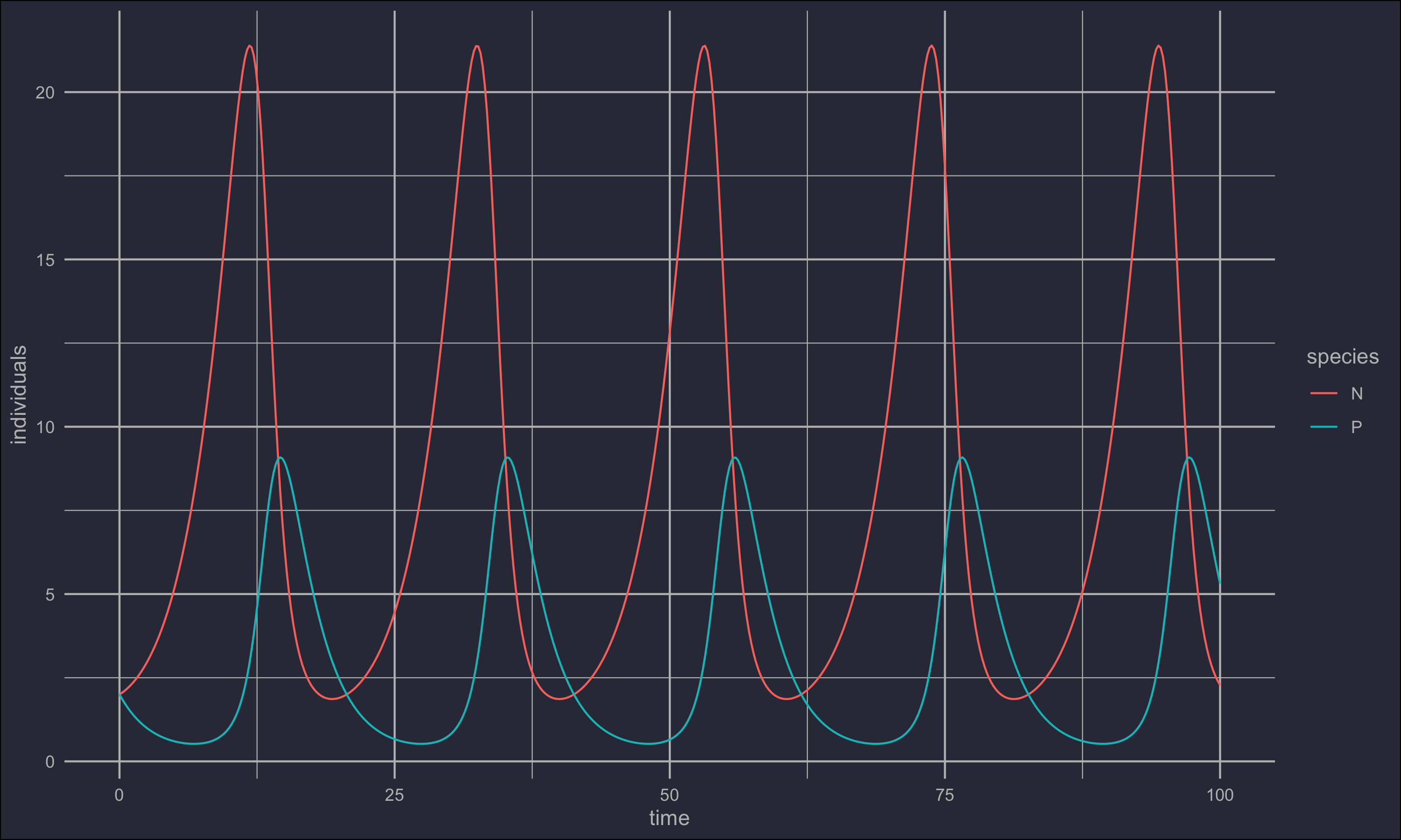
ggplot(sol2) + 
  geom_line(aes(time, individuals, colour = species))+
   theme_minimal() +
  theme(
    plot.background = element_rect(fill = rgb(.2,.21,.27)),
    text = element_text(colour = 'grey'), 
    axis.text = element_text(colour = 'grey'), 
    panel.grid = element_line(colour = 'grey')
  )

Another way of visualising the solution to the ODE system is by plotting each population on each axis.

ggplot(sol) + 
  geom_path(aes(N, P), colour = 'red', size = 1)+
   theme_minimal() +
  theme(
    plot.background = element_rect(fill = rgb(.2,.21,.27)),
    text = element_text(colour = 'grey'), 
    axis.text = element_text(colour = 'grey'), 
    panel.grid = element_line(colour = 'grey')
  )

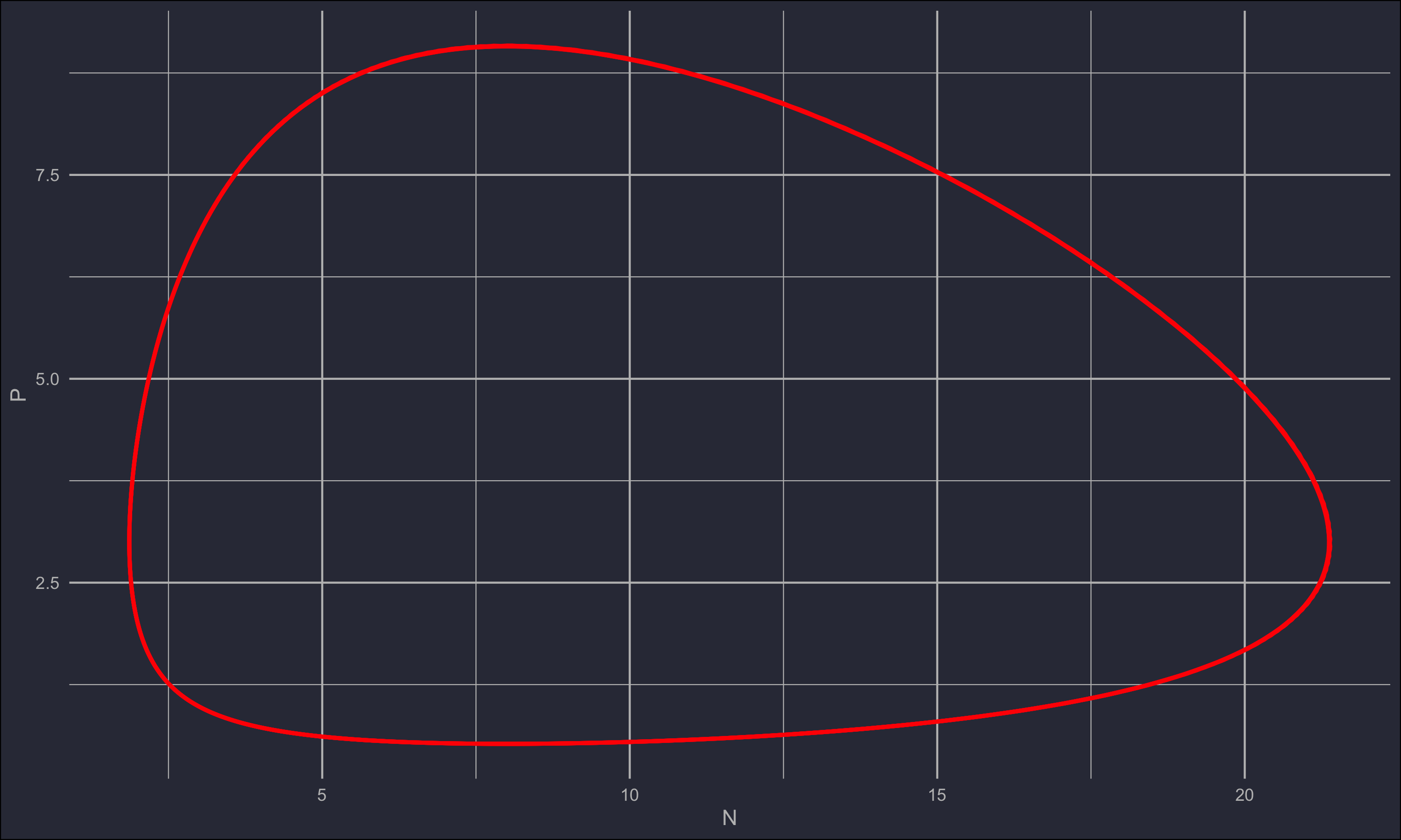
While you may have already guessed it, this plot shows that the population densities are cyclical.

Incorporating logistic growth

Let's now incorporate the logistic growth function in the prey population to see the effect (assuming a carrying capacity of ).

parameters <- c(r = 0.3, a = 0.1, b = 0.4, e = 0.5, K = 15)
state <- c(N = 2, P = 2)
lotka_volterra_K <- function(t, state, parameters) {
  with(as.list(c(state, parameters)), {
    dN <-  (1 - N/K)*r*N - a*N*P
    dP <-  e*a*N*P - b*P
    list(c(dN, dP))
  })
}

times <- seq(0, 100, by = 0.2)
sol = as.data.frame(
  ode(y = state, times = times, func = lotka_volterra_K, parms = parameters)
)

soll = gather(sol, species, individuals, -time)

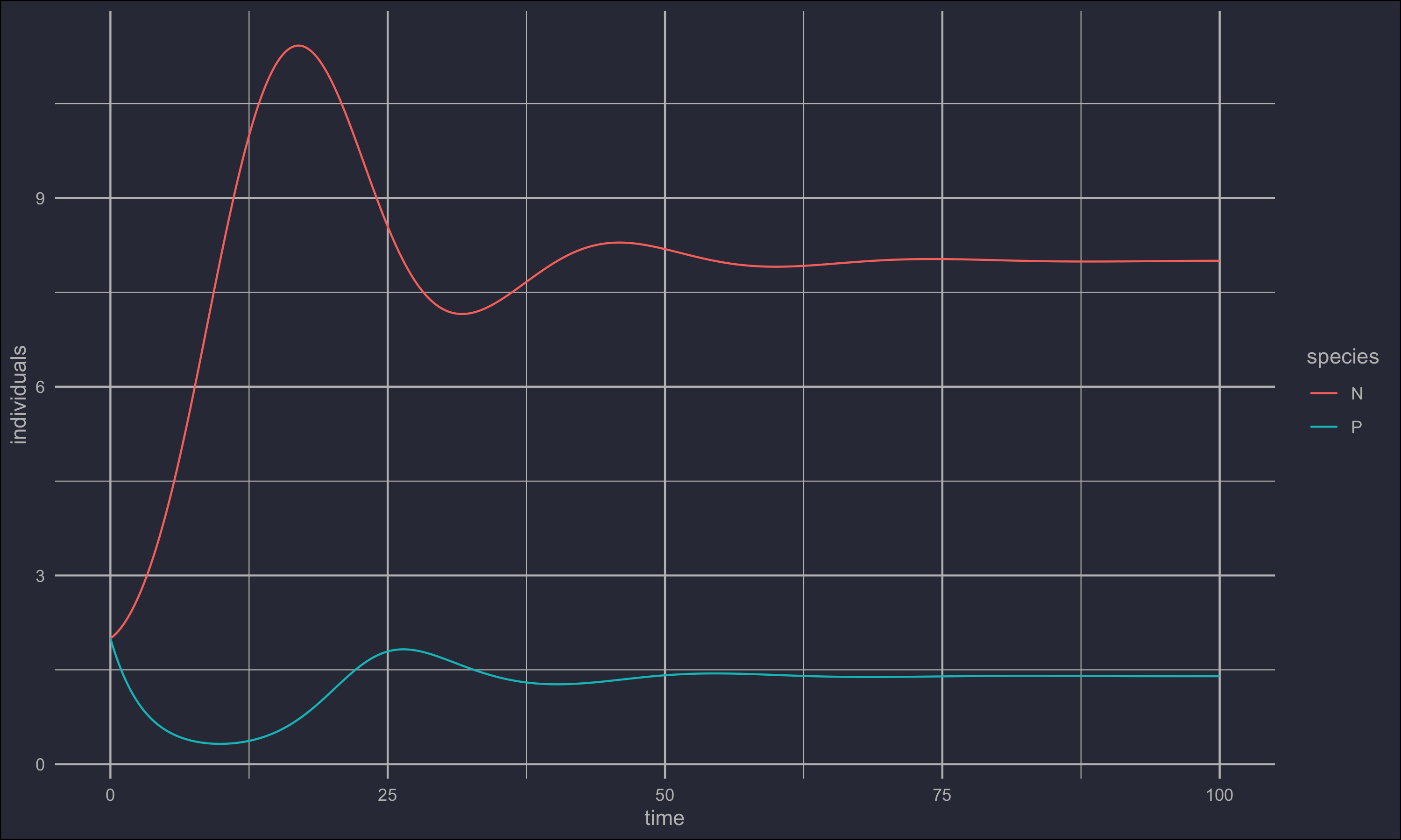
ggplot(soll) + 
  geom_line(aes(time, individuals, colour = species))+
   theme_minimal() +
  theme(
    plot.background = element_rect(fill = rgb(.2,.21,.27)),
    text = element_text(colour = 'grey'), 
    axis.text = element_text(colour = 'grey'), 
    panel.grid = element_line(colour = 'grey')
  )

And now plotting vs. with rainbow time.

ggplot(sol) + 
  geom_path(aes(N, P, colour = time), size = 1)+
   theme_minimal() +
  theme(
    plot.background = element_rect(fill = rgb(.2,.21,.27)),
    text = element_text(colour = 'grey'), 
    axis.text = element_text(colour = 'grey'), 
    panel.grid = element_line(colour = 'grey')
  ) + 
  scale_color_gradientn(colours = rainbow(9))

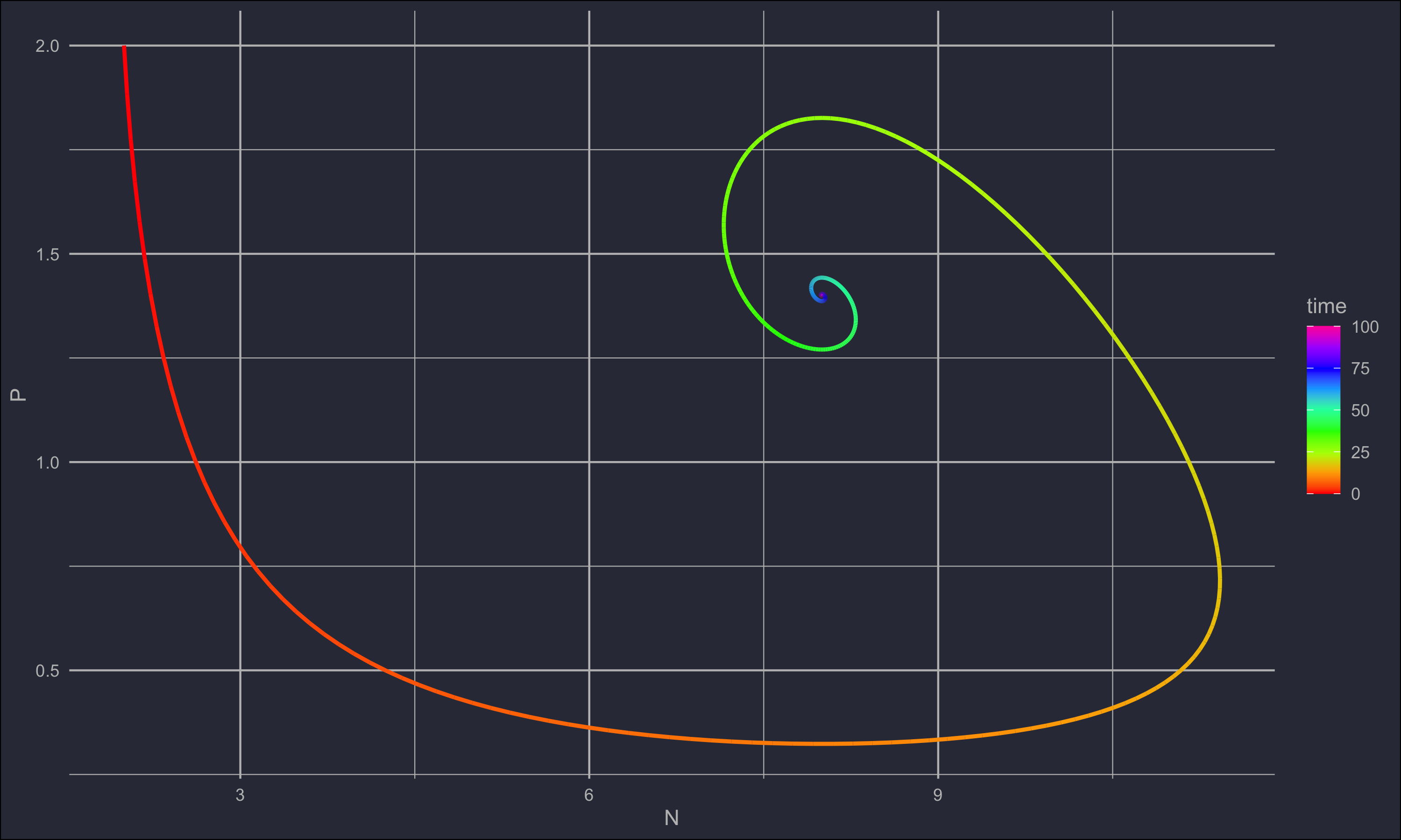
Wow! Now we have dampening and a stable state!

> sol[nrow(sol),]
    time        N        P
501  100 8.002624 1.398892

At first glance, these simulations look kind of reasonable. Our prey population grows exponentially as before, but now reaches a point of decline as the predator population builds up. Population numbers can be cyclical, like in our first example, or may approach a steady state, like in our second example.

One of the side-effects of working with continuous variables like and is that we get "fractions" of individuals, which is not realistic in the strict sense. For example, what does it mean when the predator population dips below 1? Should the population go extinct? This highlights another other issue around having assumed a deterministic system, rather than a stochastic one.

In this example, we used a concrete case where parameters, such as reproduction, or ingestion efficiency were fixed, but there is a large literature that explores the behaviour of such systems in abstract terms. What combination of parameters while lead to particular system behaviour? For example, we might want to solve the steady state of the system in general terms. For interested readers, I can highly recommend the book by the legendary John Maynard-Smith for a clear overview of some classic models, Models in Ecology.

Source code is available here