Modelling density dependent (logistic) population growth
Let's derive some more population growth functions!
One way to set un upper limit on population growth is to scale the growth rate
When
Numerical solution
Before we solve this equation with maths (analytically), let's solve it using computers (numerically) for
library(tidyverse)
library(deSolve)
parameters <- c(r = 0.3, K = 100)
state <- c(N = 2)
logistic <- function(t, state, parameters) {{
  with(as.list(c(state, parameters)), {{
    dN <-  (1 - N / K) * (r * N )
    list(dN)
  }})
}}
times <- seq(0, 50, by = 0.2)
sol = as.data.frame(
  ode(y = state, times = times, func = logistic, parms = parameters)
)
ggplot(sol) +
  geom_line(aes(time, N), col = 'red')+
   theme_minimal() +
  theme(
    plot.background = element_rect(fill = rgb(.2,.21,.27)),
    text = element_text(colour = 'grey'),
    axis.text = element_text(colour = 'grey'),
    panel.grid = element_line(colour = 'grey')
  )

Wow! That was easy.
Analytical solution
Now that we've seen the pretty curve, let's use our excitement to try and describe the curve with a single equation without derivatives (solve the differential equation for
First, separate the variables.
Now we want to split up the fraction into something more manageable so we assume there exists some
When
Now substituting
Thus we have:
Now integrate both sides:
The part
From here we can finish the original integration.
As N is strictly positive we can remove the absolute operators. Remembering your logarithm rules
We really just want one
Back to solving for
Substitute in the constant we solved for earlier.
And simplify by multiplying through by
Let plot it!
r = 0.3
K = 100
N0 = 2
time <- seq(0, 50, by = 0.2)
sol = data.frame(
  time,
  N = K*N0/(N0 + (K - N0)*exp(-r*time))
)
ggplot(sol) +
  geom_line(aes(time, N), col = 'red')+
   theme_minimal() +
  theme(
    plot.background = element_rect(fill = rgb(.2,.21,.27)),
    text = element_text(colour = 'grey'),
    axis.text = element_text(colour = 'grey'),
    panel.grid = element_line(colour = 'grey')
  )
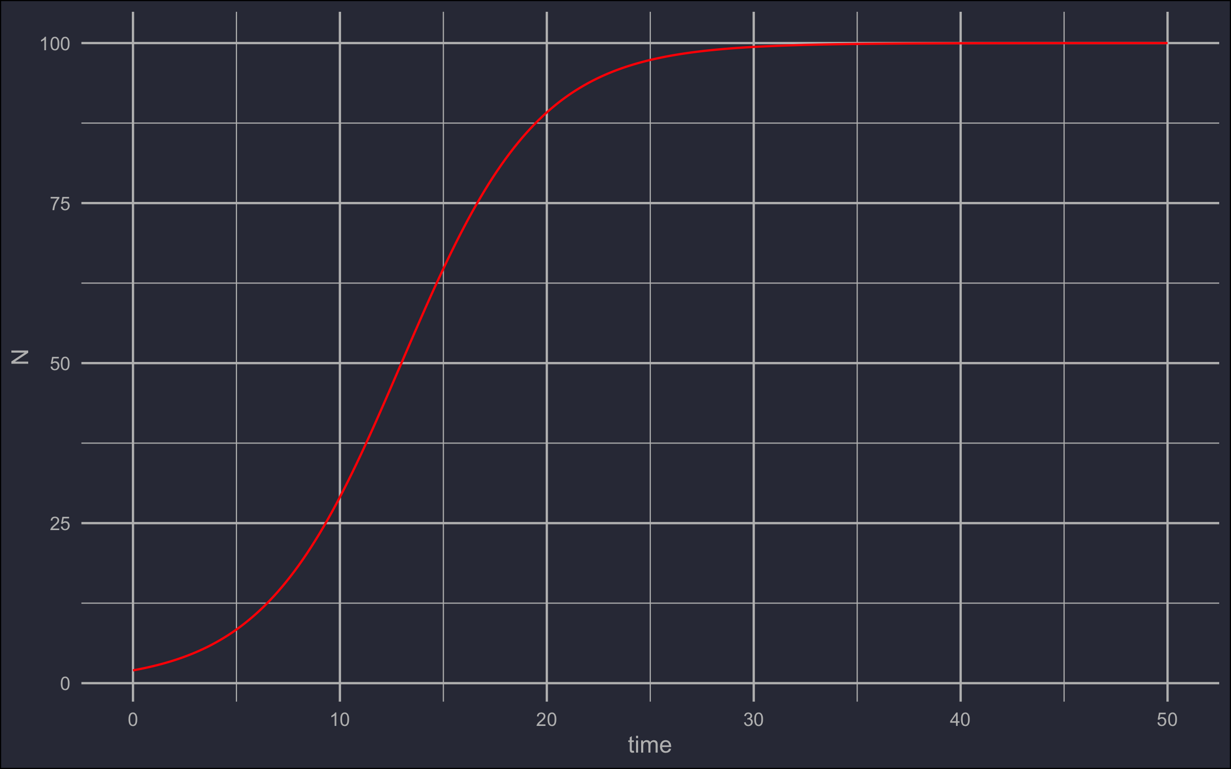
All that calculus for the same line deSolve gave us...