Modelling unconstrained population growth rates

Let's derive some population growth functions!

Populations grow. They grow positively, if rates of reproduction > mortality, or negatively, if reproduction < mortality. For an unconstrained population of size (see here for the contained case), this difference in per capita reproduction and mortality is referred to as the intrinsic growth rate, and has the units individuals per individual per time . The value of is a constant if the age-distribution is constant (e.g. the proportion of reproductively active individuals in the population does not change). Taking as constant, the change in population size with time is simply:

This is a rudimentary first-order differential equation which can be solved in a few simple steps.

Solving for at :

While the parameter hopefully makes conceptual sense, it is not straightforward to measure for a given species, as it will depend on the age structure (all juveniles means no reproduction), resource availability (food for growth), and environmental temperature (slow cold ectotherms). The age structure is assumed to be in a steady state, i.e. the relative proportion of different age classes does not change. Likewise, resource availability and other environmental conditions such as temperature are also taken as fixed. Steady state can be illustrated with a simple transition matrix model. Although there are initially 1000 individuals in the first age class (e.g. a mass hatching event triggered by rain), the age classes eventually stabilise.

library(tidyverse)

trans = matrix(
  c(0.00, 0.50, 0.00,
    0.00, 0.00, 0.50,
    4.00, 0.00, 0.10),
  ncol = 3,byrow = T
  )

rownames(trans) = c('V1','V2','V3')

colnames(trans) = c('V1','V2','V3')

> trans
   V1  V2  V3
V1  0 0.5 0.0
V2  0 0.0 0.5
V3  4 0.0 0.1

Tmax = 200

N = matrix(rep(0, Tmax*3), nrow = 3)

N[1,1] = 1000

for(t in 2:Tmax) N[, t] = N[, t-1] %*% trans

# plot

ages = as.data.frame(t(N))

ages$total = rowSums(ages)

ages$t = 1:Tmax

agesl = gather(ages, age.class, value, -t, - total)

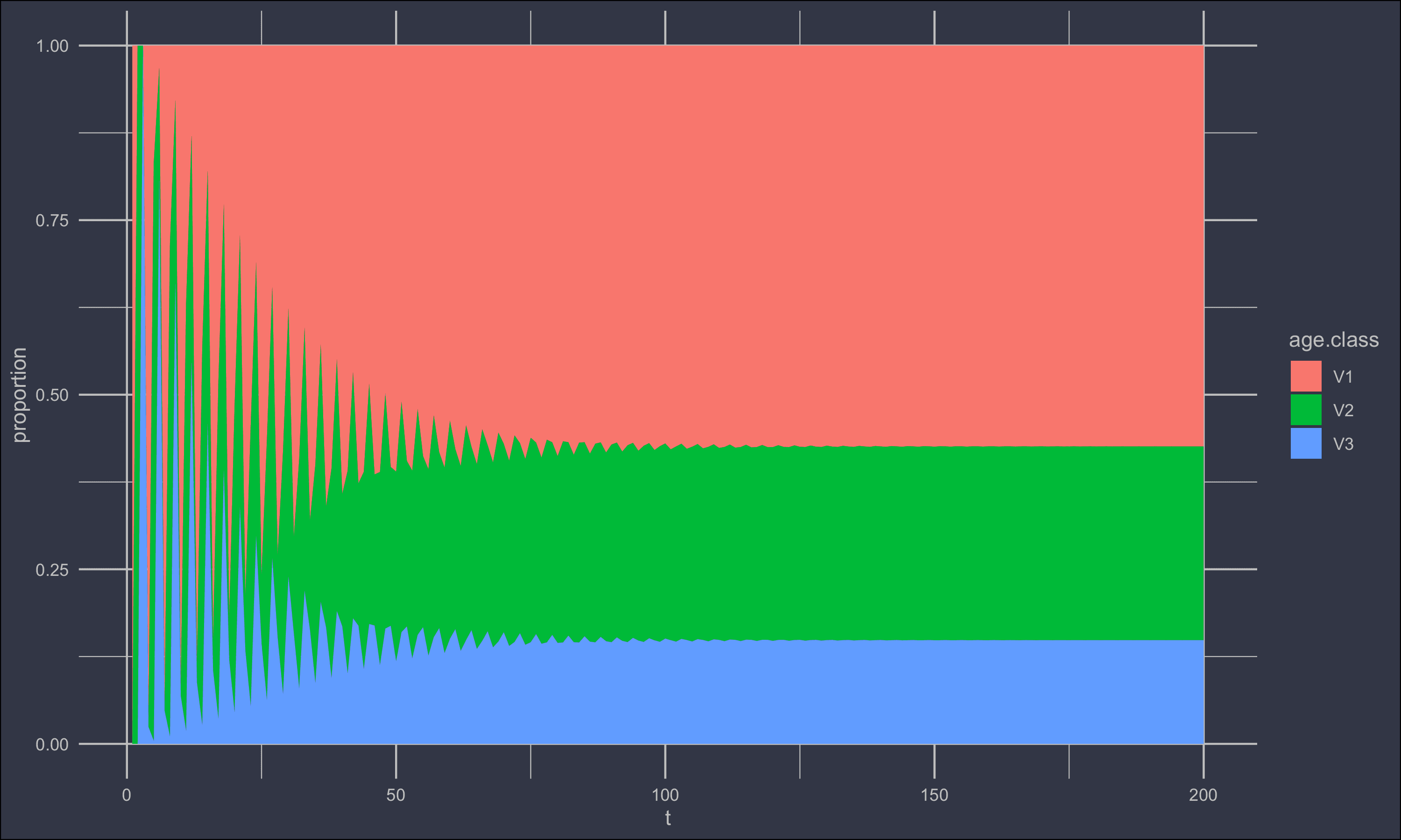
ggplot(agesl) + 
  geom_area(aes(t, value/total, fill = age.class)) +
  ylab('proportion')+
  theme_minimal() +
  theme(
    plot.background = element_rect(fill = rgb(0.2,0.21,0.27)),
    text = element_text(colour = 'grey'), 
    axis.text = element_text(colour = 'grey'), 
    panel.grid = element_line(colour = 'grey')
  )

Regressing population vs. time

There are a number of ways that can be measured, but they all rely on the above assumptions.

The most direct way to access is to look at how an unconstrained growing population changes through time. Let's use the numbers from our previous matrix model simulation.

df = data.frame(
      t = 0:(Tmax-1),
      N = colSums(N)
     )

To estimate through regression, notice that a log tranformation of the growth function results in:

This is a linear regression with an intercept and slope which we can recover through fitting a simple linear model.

lm1 = lm(log(N) ~ t , data = df)

coef(lm1)

> coef(lm1)
(Intercept)           t 
 6.30299077  0.03407767 

# plot 

df$pred = predict(lm1)

ggplot(df) +
  geom_line(aes(t,N), colour = 'red', alpha = 0.5) + 
  geom_line(aes(t,exp(pred)), colour = 'grey') + 
  theme_minimal() +
  theme(
    plot.background = element_rect(fill = rgb(.2,.21,.27)),
    text = element_text(colour = 'grey'), 
    axis.text = element_text(colour = 'grey'), 
    panel.grid = element_line(colour = 'grey')
  ) +
  scale_y_log10()
  

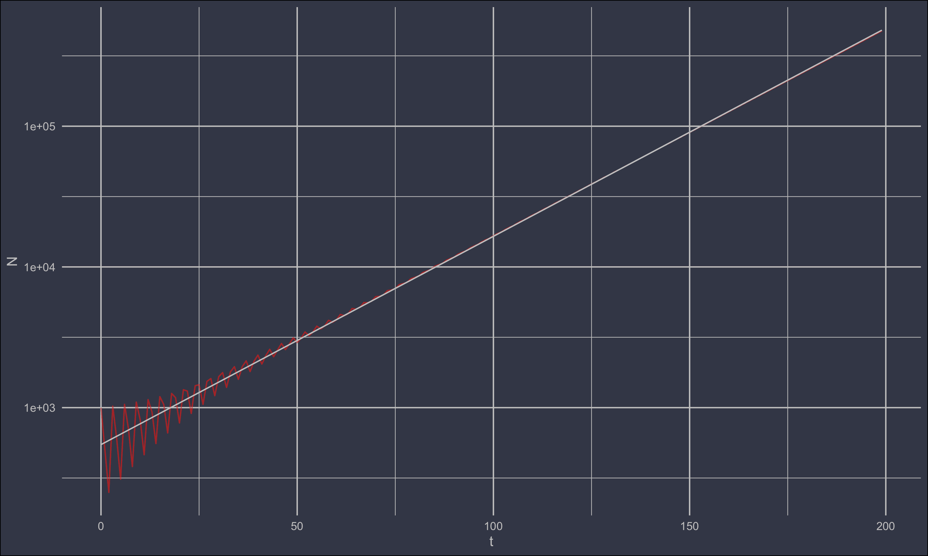
Notice that the recovered intercept exp(coef(lm1)[1]) = r round(exp(coef(lm1)[1])) was actually lower than the real values of 1000. This was due to the age distribution not being in steady state, and the population not growing properly exponential.

Now let's try and run the same matrix model simulation but with the 1000 individuals distributed across age classes at the steady state proportions.

N1_stable = 1000*N[,Tmax]/sum(N[,Tmax])

N = matrix(rep(0, Tmax*3), nrow = 3)

N[,1] = N1_stable 

for(t in 2:Tmax) N[, t] = N[, t-1] %*% trans

df = data.frame(
      t = 0:(Tmax-1),
      N = colSums(N)
     )

lm1 = lm(log(N) ~ t , data = df)

> coef(lm2)
(Intercept)           t 
 6.90777973  0.03388836 

After exponentiating the intercept we are able to recover the initial population size.

> exp(coef(lm2)[1])
(Intercept) 
   1000.024 

Measuring vital rates and building a life table

Old school population demographers also built life tables for a cohort of individuals followed through life, which include direct measurements of mortality, and reproduction to calculate .

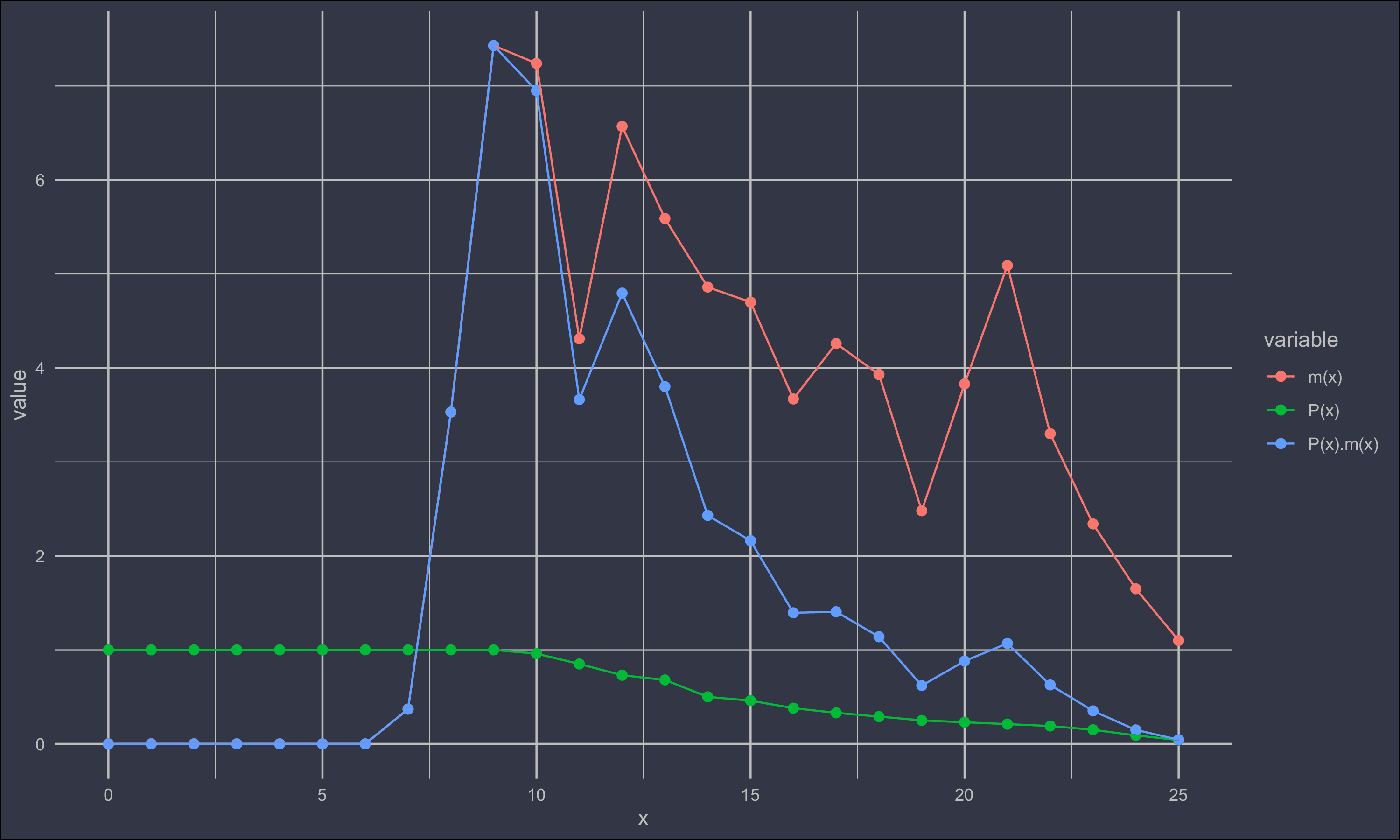
Let's use an example published by Carey and Bradley of the Atlantic Spider mite. The below table shows for each day the proportion surviving and mean daily reproduction rate per individual for a synchronised cohort through time starting at egg lay.

mite = read_csv('data/AtlanticSpiderMite_CareyBradley1982.csv')

> mite
# A tibble: 26 × 3
       x `P(x)` `m(x)`
   <dbl>  <dbl>  <dbl>
 1     0      1   0   
 2     1      1   0   
 3     2      1   0   
 4     3      1   0   
 5     4      1   0   
 6     5      1   0   
 7     6      1   0   
 8     7      1   0.37
 9     8      1   3.53
10     9      1   7.43
# … with 16 more rows
# ℹ Use `print(n = ...)` to see more rows

Firstly, we estimate net generational reproduction . As not all individuals will reproduce at , i.e. some will die, this value is scaled by . Now let's plot mortality and reproduction data. But how fast does a population grow by this factor?

# plot 

mite$`P(x).m(x)` = mite$`P(x)`*mite$`m(x)`

dw = mite %>% gather(variable, value, -x)

ggplot(dw) +
  geom_point(aes(x,value, colour = variable), size = 2) +  
  geom_line(aes(x,value, colour = variable)) +
  theme_minimal() +
  theme(
    plot.background = element_rect(fill = rgb(.2,.21,.27)),
    text = element_text(colour = 'grey'), 
    axis.text = element_text(colour = 'grey'), 
    panel.grid = element_line(colour = 'grey')
  )
  

An analytical estimate of r from this data relies on the Lotka equation.

Here we can set where

Substituting into the Lotka equation and recognising we get :

Alternatively, we can solve this equation numerically.

Source code available here

Carey, J.R. and Bradley, J.W., 1982. Developmental rates, vital schedules, sex ratios and life tables for Tetranychus urticae, T. turkestani and T. pacificus (Acarina: Tetranychidae) on cotton. Acarologia, 23(4), pp.333-345.