Fitting simple Bayesian glm models with stan in R
We can visually show the difference in a Bayesian vs a frequentist approach to statistical inference using a simple coin toss example.
Here, we flip a coin 200 times with
n <- 200
set.seed(1234)
outcomes <- cumsum(rbinom( n, 1, 0.5 ))
samples <- 1:n
p_hat = outcomes/samples
sd_p =  sqrt( 0.5 * (1 - 0.5) / samples )
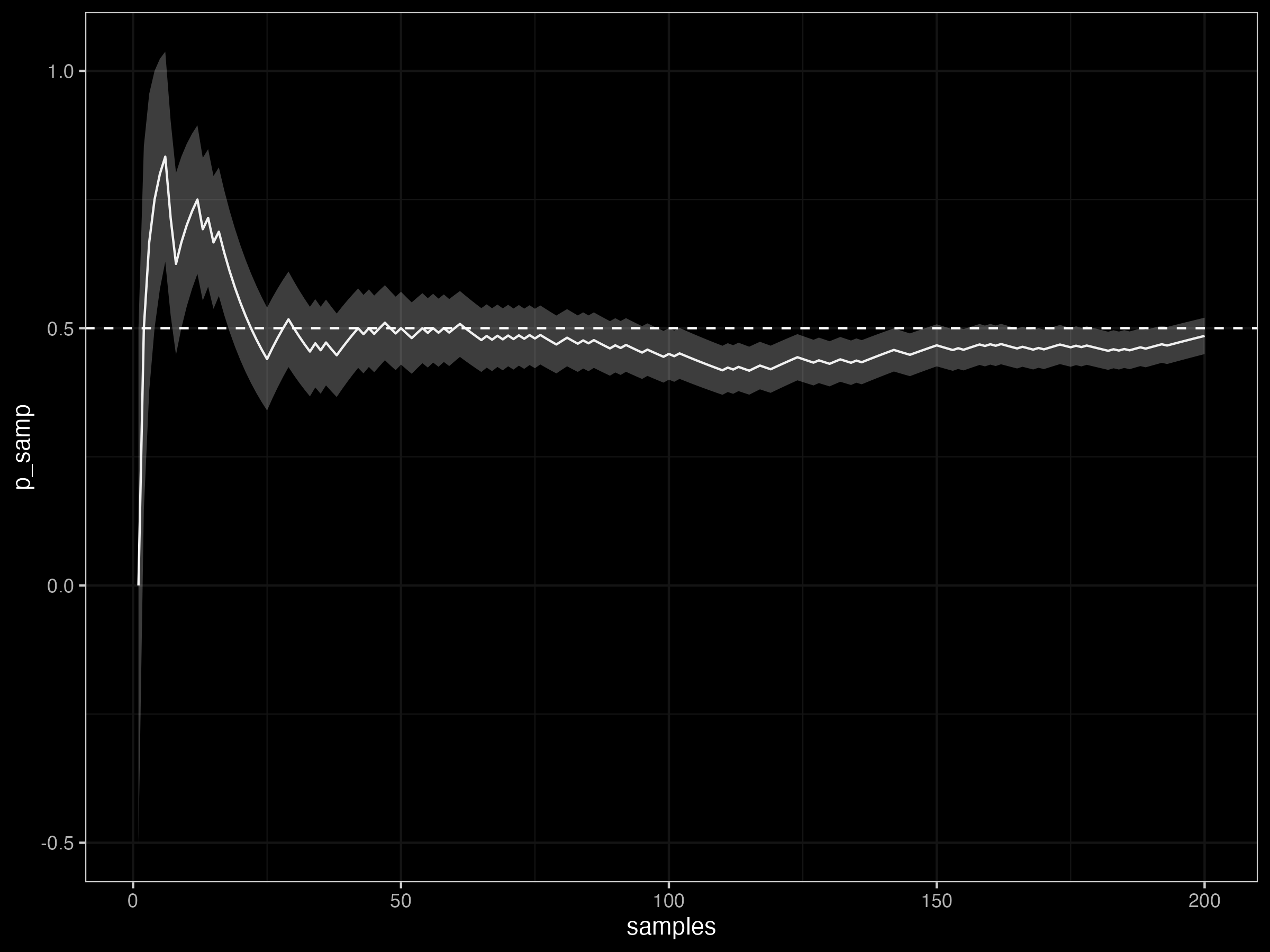
Under a frequentist perspective, we might see that the more coin flips we make, the closer our sample estimate converges to the true proportion of 0.5 and the smaller the sd of our sample estimate
ggplot() +
    geom_line(aes(samples, p_hat)) +
    geom_ribbon(aes(samples, ymin=p_hat - sd_p,
                             ymax=p_hat + sd_p), alpha=0.3) +
    geom_hline(yintercept = 0.5, linetype=2) +
    dark_theme_bw()
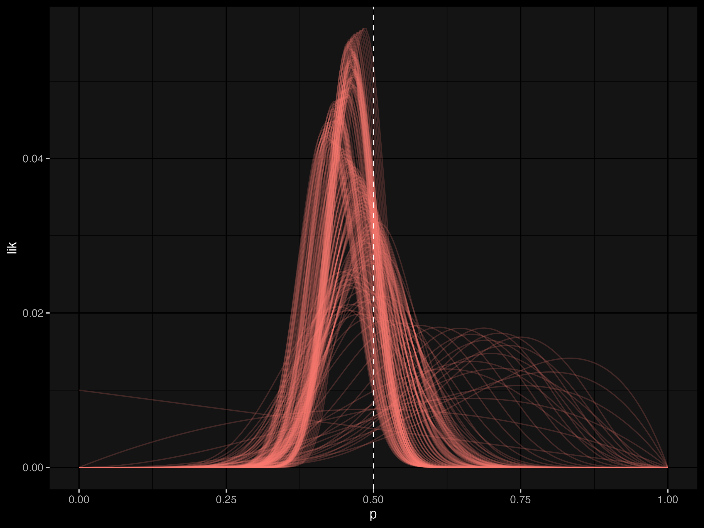
But another way of seeing the coin is as probability density function where
p <- seq(0, 1, length = n)
tibble(samples, outcomes) %>%
    group_by(samples, outcomes) %>%
    expand_grid(p) %>%
    rowwise %>%
    mutate(log_lik = sum(log(dbinom(outcomes, samples, p)))) %>%
    mutate(lik = exp(log_lik)) %>%
    group_by(samples) %>%
    mutate(lik = lik/sum(lik)) %>%
    ggplot() +
        geom_line(aes(p, lik, group=samples, color='white'), alpha=0.2) +
        guides(color = "none") +
        geom_vline(xintercept = 0.5, linetype=2) +
        theme_bw() +
        dark_theme_gray()
The Bayesian approach was a bit more computationally intensive, as you would notice if you tried to make these plots. This is due to estimating the probability density of each model parameter.
Fitting a glm with glm
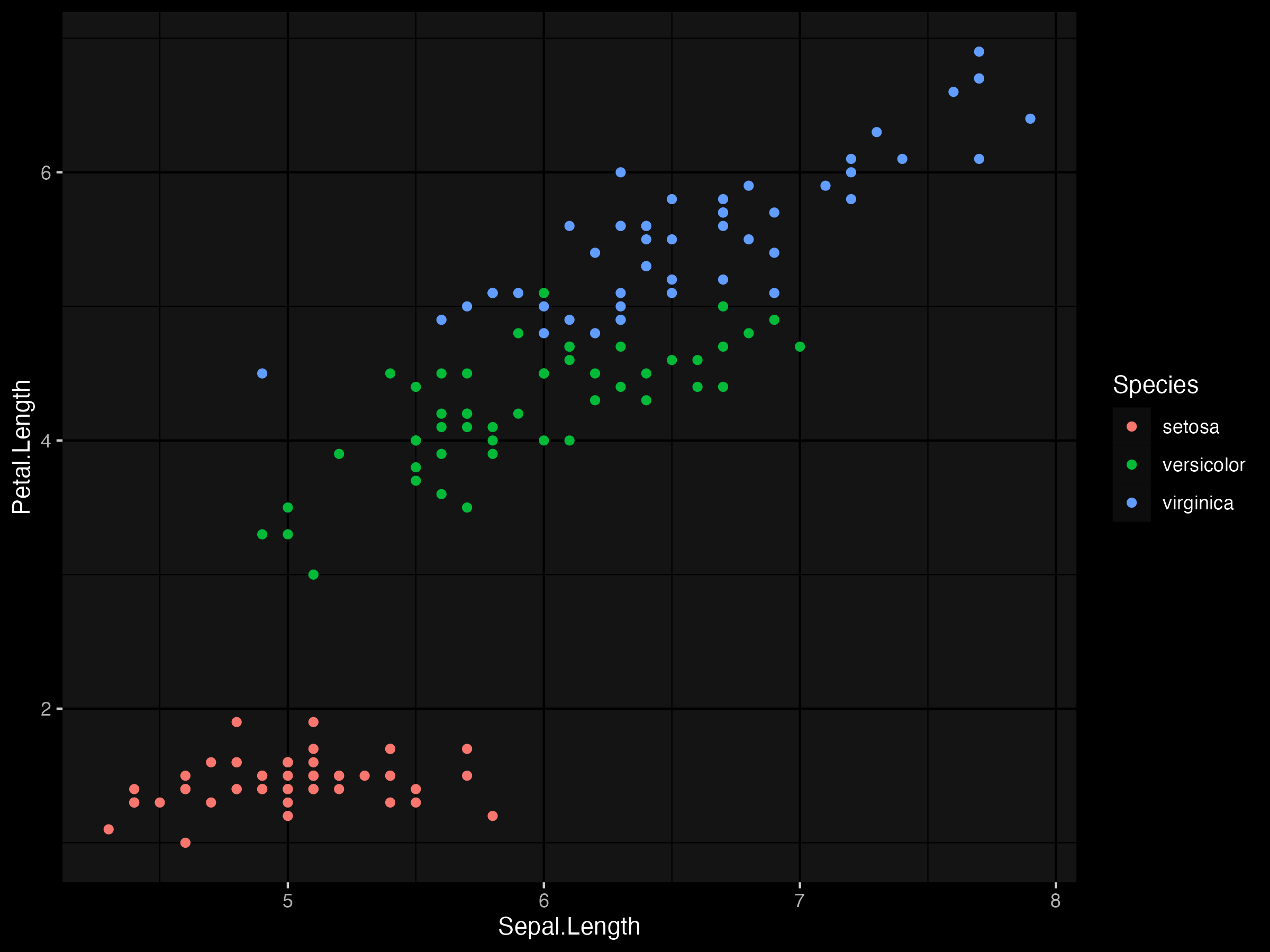
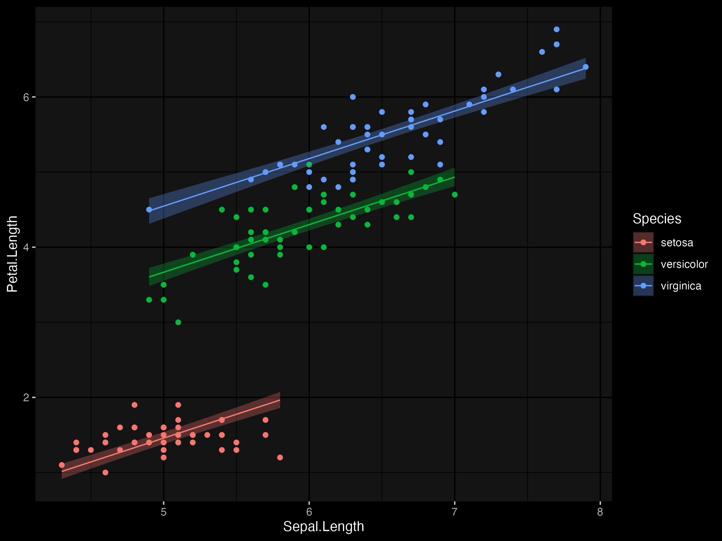
Here we use the iris data set bundled with R, which can be visualised as follows.
data(iris)
d <- as.data.frame(iris)

p <- ggplot(d, aes(Sepal.Length, Petal.Length, color = Species)) +
    geom_point() +
    dark_theme_grey()
p
First, we start with a simple linear regression but use the glm function with the argument family=gaussian to make to approach more general other model families (binomial, poisson, etc.). I find it is always handy to know multiple ways to fit a model.
m1 <- glm(Petal.Length ~ Sepal.Length + Species,
    family = gaussian,
    data = d
)

m1_pred <- predict(m1, se.fit = TRUE) %>%
    as_tibble() %>%
    mutate(
        lower = fit - 1.96 * se.fit,
        upper = fit + 1.96 * se.fit
    )
p +
    geom_line(aes(y = m1_pred$fit)) +
    geom_ribbon(aes(ymin = m1_pred$lower, ymax = m1_pred$upper, fill = Species),
        alpha = 0.3,
        color = NA
    )

> summary(m1)

Call:
glm(formula = Petal.Length ~ Sepal.Length + Species, family = gaussian,
    data = d)

Deviance Residuals:
     Min        1Q    Median        3Q       Max
-0.76390  -0.17875   0.00716   0.17461   0.79954

Coefficients:
                  Estimate Std. Error t value Pr(>|t|)
(Intercept)       -1.70234    0.23013  -7.397 1.01e-11 ***
Sepal.Length       0.63211    0.04527  13.962  < 2e-16 ***
Speciesversicolor  2.21014    0.07047  31.362  < 2e-16 ***
Speciesvirginica   3.09000    0.09123  33.870  < 2e-16 ***
---
Signif. codes:  0 ‘***’ 0.001 ‘**’ 0.01 ‘*’ 0.05 ‘.’ 0.1 ‘ ’ 1

(Dispersion parameter for gaussian family taken to be 0.07984347)

    Null deviance: 464.325  on 149  degrees of freedom
Residual deviance:  11.657  on 146  degrees of freedom
AIC: 52.474

Number of Fisher Scoring iterations: 2
Fitting a glm with rstan
One of the downsides of using rstan is the manual data preparation required for model fitting. While there are handy packages like rstanarm which help to reduce this overhead, it is not too difficult to start from scratch if we use a couple of tricks.
Using the model.matrix function is a handy way to build a covariate matrix which will save us having to the update the model defined in .stan and data passed to the stan() each time we tweak the model.
> model.matrix(m1)
    (Intercept) Sepal.Length Speciesversicolor Speciesvirginica
1             1          5.1                 0                0
2             1          4.9                 0                0
3             1          4.7                 0                0
4             1          4.6                 0                0
5             1          5.0                 0                0
//...
146           1          6.7                 0                1
147           1          6.3                 0                1
148           1          6.5                 0                1
149           1          6.2                 0                1
150           1          5.9                 0                1
Another handy tool is the lookup() function from stan, which can help find a suitable probability density function in stan.
> lookup(dnorm)
          StanFunction
374 normal_id_glm_lpmf
375 normal_id_glm_lpmf
376      normal_id_glm
379        normal_lpdf
380             normal
                                                       Arguments ReturnType
374   (vector y , matrix x, real alpha, vector beta, real sigma)       real
375 (vector y , matrix x, vector alpha, vector beta, real sigma)       real
376                                                            ~       real
379                            (reals y , reals mu, reals sigma)       real
380                                                            ~       real
Here we select the normal function and construct our .stan file as follows:
//lm_model.stan

data {
  int <lower = 0> N;
  vector [N] y ;
  int<lower=0> K;
  matrix[N, K] X;
}

parameters {
  vector [K] beta;
  real <lower=0> sigma;
}

model {
    y ~ normal_lpdf(beta*X, sigma);
}
We then construct a list of the data that matches the structure defined in the stan file and fit the stan model.
stan_data <- list(
    N = nrow(mat),
    y = d$Petal.Length,
    K = ncol(mat),
    X = mat
)

m2 <- stan(
    file = "lm_model.stan",
    data = stan_data,
    warmup = 500,
    iter = 3000,
    chains = 4,
    cores = 4,
    thin = 1,
    seed = 123
)
If we check the model parameter estimates, they are very close to those estimated above by lm.
> print(m2, probs = c(0.025, 0.975))
Inference for Stan model: lm_model.
4 chains, each with iter=3000; warmup=500; thin=1;
post-warmup draws per chain=2500, total post-warmup draws=10000.

          mean se_mean   sd   2.5%  97.5% n_eff Rhat
beta[1]  -1.71    0.00 0.23  -2.16  -1.26  2765    1
beta[2]   0.63    0.00 0.05   0.54   0.72  2564    1
beta[3]   2.21    0.00 0.07   2.07   2.35  3282    1
beta[4]   3.09    0.00 0.09   2.90   3.27  2956    1
sigma     0.28    0.00 0.02   0.25   0.32  5616    1
lp__    -25.02    0.03 1.54 -28.81 -22.93  3724    1

Samples were drawn using NUTS(diag_e) at Fri Aug 12 10:02:49 2022.
For each parameter, n_eff is a crude measure of effective sample size,
and Rhat is the potential scale reduction factor on split chains (at
convergence, Rhat=1).
Constructing the prediction interval is a little different to above. Because we don't have direct estimates to the uncertainty in parameter estimates, it must be accessed via sampling the posterior distribution. So we take a bunch of samples and calculate the appropriate quantiles of interest (e.g. 95% credible intervals).
e <- rstan::extract(m2)
str(e)

dim(e$beta)
dim(mat)
pred_post <- e$beta %*% t(mat)
pred <- apply(pred_post, 2, function(x) quantile(x, c(0.025, 0.5, 0.975)))
m2_pred <- d %>%
    transmute(
        lower = pred[1, ],
        mu    = pred[2, ],
        upper = pred[3, ]
    )
p +
    geom_line(aes(y = m2_pred$mu)) +
    geom_ribbon(aes(ymin = m2_pred$lower, ymax = m2_pred$upper, fill = Species),
        alpha = 0.3,
        color = NA
    )
While this sounds like more work, in practice it is a flexible approach that can allow us to very quickly make inference on any derived or compound parameters.
Extensions to other model families (binomial model)
Thanks to a little bit of linear algebra used with model.matrix() and the
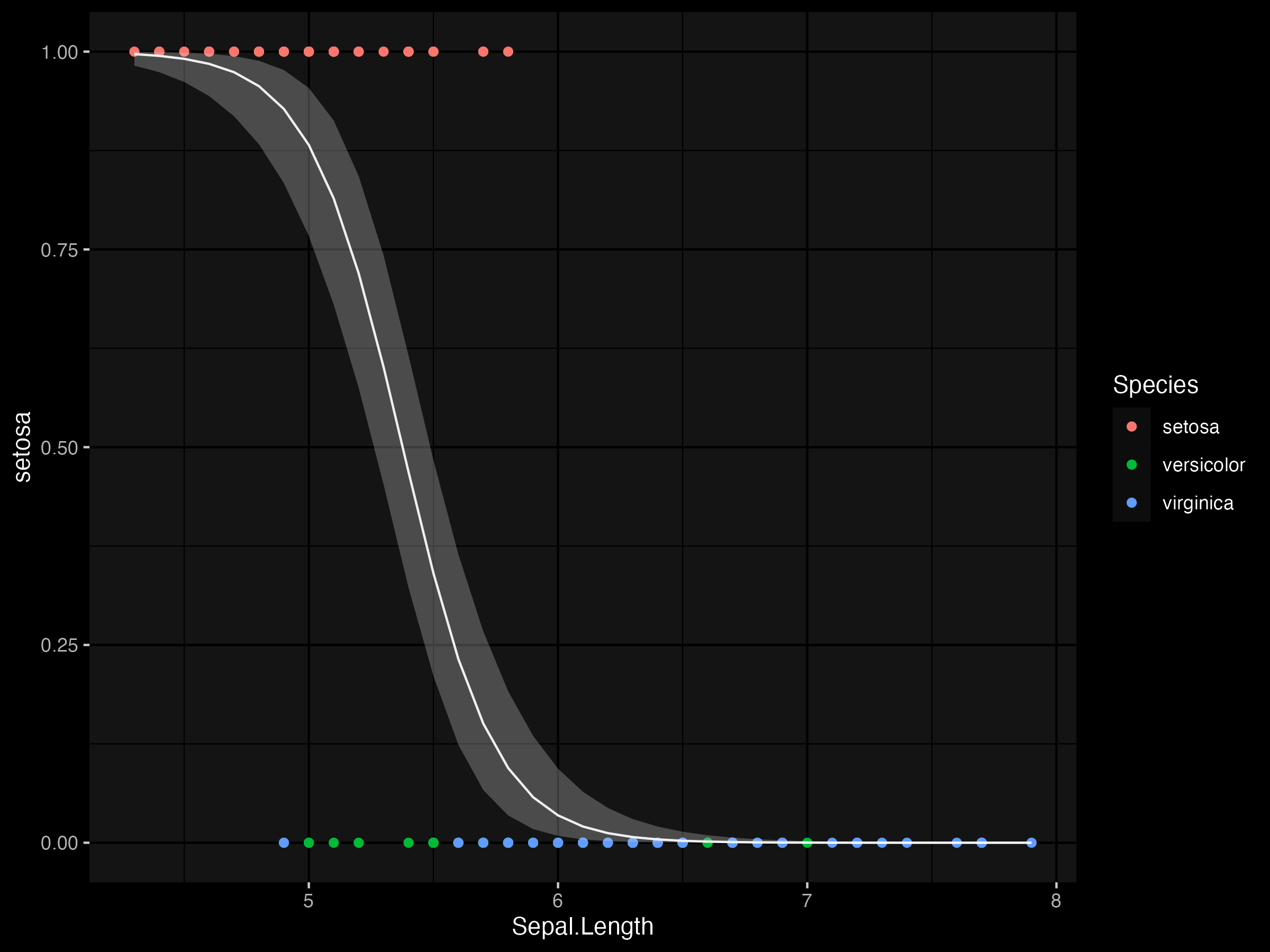
For the binomial data we will predict the plant species setosa from the Sepal.Length variable.
d2 <- d %>%
    mutate(setosa = as.integer(Species == "setosa"))
There are just a few changes to make.
Fit a binomial glm.
glm2 <- glm(setosa ~ Sepal.Length, data = d2, family = binomial(link = "logit"))
The fitted values can be transformed back to the real scale using the inverse logit function
ilogit = function(x) exp(x)/(1+exp(x))
Update the outcome variable (1 = setosa; 0 otherwise).
stan_data2 <- list(
    # ...
    y = d2$setosa,
    # ...
)
Update the stan file.
// logit_model.stan
data {
  int <lower = 0> N;
  int<lower=0,upper=1> y[N];
  int<lower=0> K;
  matrix[N, K] X;
}

parameters {
  vector [K] beta;
}

model {
    y ~ bernoulli_logit(X*beta);
}
And that's it.