Testing differences in dose responses in two populations
Dose response are used in a variety of situations where the impact of exposure, dose, or concentration on some measurement endpoint is of interest.
Dose responses in ecology
For a given species, a simple mortality response to environmental conditions can be represented with the probabilistic outcome (death), which occurs with probability
library(tidyverse)
library(rstan)
d = read_csv('data/DoseResponseMaino2018.csv', col_types = 'ccniii') %>%
  mutate(dead = dead + incapacitated) %>%
  dplyr::select(-incapacitated) %>%
  group_by(treatment, pop, dose) %>%
  summarise_all(sum) %>%
  mutate(total = dead + alive) %>%
  filter(dose != 0)
> d
# A tibble: 14 × 6
# Groups:   treatment, pop [2]
   treatment pop           dose alive  dead total
   <chr>     <chr>        <dbl> <int> <int> <int>
 1 omethoate control      0.007    52     0    52
 2 omethoate control      0.07     49     0    49
 3 omethoate control      0.7      53     3    56
 4 omethoate control      7        36    13    49
 5 omethoate control     70         0    51    51
 6 omethoate control    700         0    48    48
 7 omethoate control   7000         0    51    51
 8 omethoate resistant    0.007    49     0    49
 9 omethoate resistant    0.07     47     0    47
10 omethoate resistant    0.7      50     0    50
11 omethoate resistant    7        51     0    51
12 omethoate resistant   70         9    37    46
13 omethoate resistant  700         4    45    49
14 omethoate resistant 7000         0    52    52
Logistic regression and the Bernoulli probability distribution
The Bernoulli mortality probability
where
With the logit link function and the linear equation specifying the relationship of binomial parameter
m1 = glm(cbind(dead, alive) ~ pop/log(dose) - 1, family = binomial('logit'),
         data = d )
We can print the model matrix can be observed using using the model.matrix function.
> model.matrix(m1)
   popcontrol popresistant popcontrol:log(dose) popresistant:log(dose)
1           1            0           -4.9618451              0.0000000
2           1            0           -2.6592600              0.0000000
3           1            0           -0.3566749              0.0000000
4           1            0            1.9459101              0.0000000
5           1            0            4.2484952              0.0000000
6           1            0            6.5510803              0.0000000
7           1            0            8.8536654              0.0000000
8           0            1            0.0000000             -4.9618451
9           0            1            0.0000000             -2.6592600
10          0            1            0.0000000             -0.3566749
11          0            1            0.0000000              1.9459101
12          0            1            0.0000000              4.2484952
13          0            1            0.0000000              6.5510803
14          0            1            0.0000000              8.8536654
The summary output tells us that one population called "resistant" appears to have a higher intercept.
> summary(m1)

Call:
glm(formula = cbind(dead, alive) ~ pop/log(dose) - 1, family = binomial("logit"),
    data = d)

Deviance Residuals:
     Min        1Q    Median        3Q       Max
-2.66626  -0.37482  -0.02094   0.29396   2.08559

Coefficients:
                       Estimate Std. Error z value Pr(>|z|)
popcontrol              -3.7440     0.6145  -6.093 1.11e-09 ***
popresistant            -5.7053     0.9141  -6.242 4.33e-10 ***
popcontrol:log(dose)     1.6188     0.2548   6.354 2.09e-10 ***
popresistant:log(dose)   1.5064     0.2253   6.686 2.29e-11 ***
---
Signif. codes:  0 ‘***’ 0.001 ‘**’ 0.01 ‘*’ 0.05 ‘.’ 0.1 ‘ ’ 1

(Dispersion parameter for binomial family taken to be 1)

    Null deviance: 817.127  on 14  degrees of freedom
Residual deviance:  28.145  on 10  degrees of freedom
AIC: 50.208

Number of Fisher Scoring iterations: 7
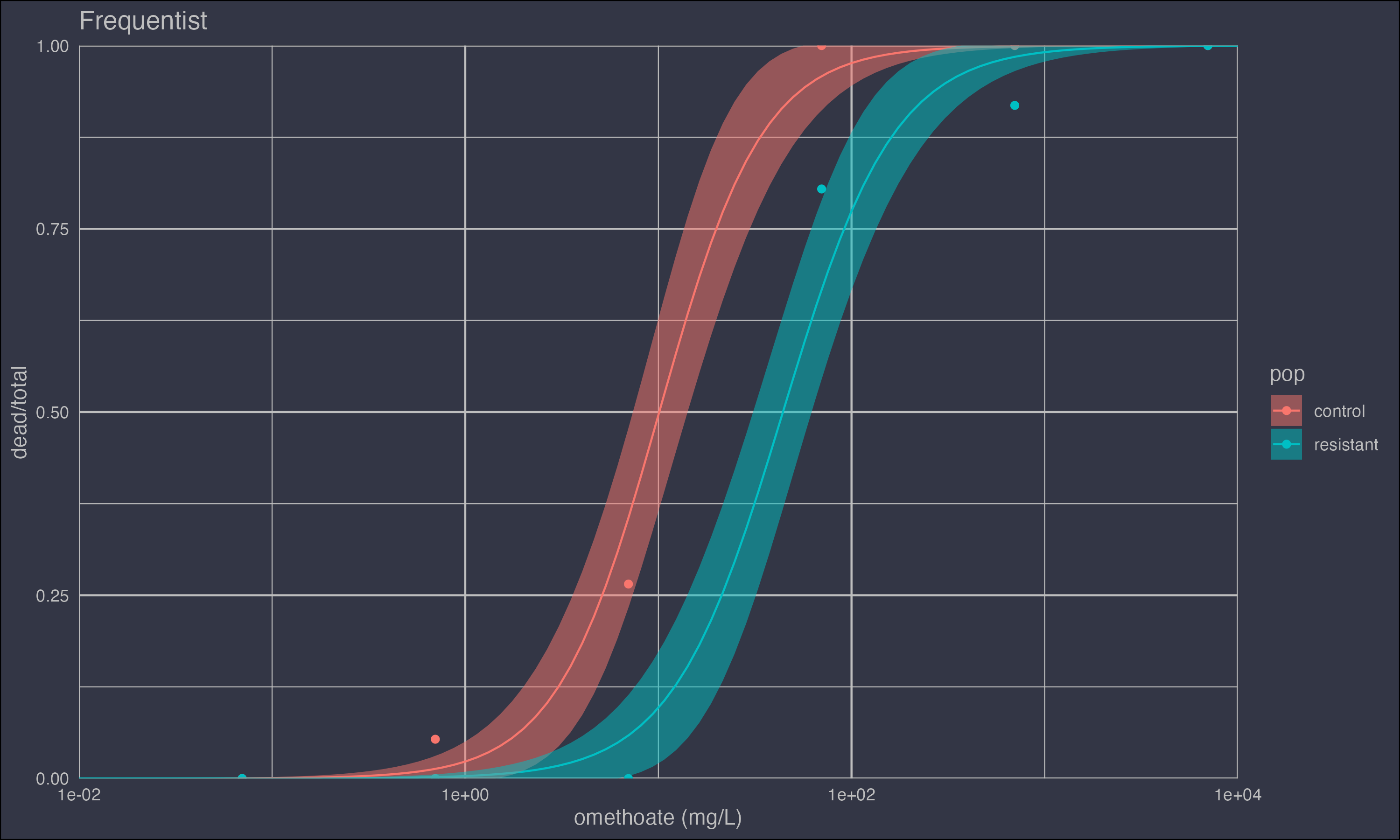
This can be confirmed visually by plotting the model with 95% confidence intervals.
m1pred = expand.grid(
  pop = c('control','resistant'),
  dose = 10^seq(-2, 4, length = 100)
)
m1pred$logdose = log(m1pred$dose)
pred = predict(m1, newdata = m1pred, type = 'response' , se.fit = TRUE)
m1pred$p = pred$fit
m1pred$se = pred$se.fit

ggplot() +
  geom_point(data = d, aes(dose, dead/total, colour = pop)) +
  geom_line(data = m1pred, aes(dose, p, colour = pop)) +
  geom_ribbon(data = m1pred,
              aes(dose, ymin = p - 1.96*se, max = p + 1.96*se, fill = pop),
              alpha = 0.5) +
  mydarktheme +
  xlab('omethoate (mg/L)') +
  ggtitle('Frequentist') +
  scale_x_log10()
We can also rearrange the data into a Bernoulli format (each row is an individual trial) using the following
db = d %>%
  rowwise() %>%
  mutate(outcome = list(rep(c(0, 1), c(alive, dead)))) %>%
  dplyr::select(-alive,-dead, -total) %>%
  unnest()
> head(db)
# A tibble: 6 × 4
# Groups:   treatment, pop [1]
  treatment pop      dose outcome
  <chr>     <chr>   <dbl>   <dbl>
1 omethoate control 0.007       0
2 omethoate control 0.007       0
3 omethoate control 0.007       0
4 omethoate control 0.007       0
5 omethoate control 0.007       0
6 omethoate control 0.007       0
The model coefficients and standard errors are the same despite our trial size changing to
m1 = glm(outcome ~ pop/log(dose) - 1, family = binomial('logit'),
         data = db )
> summary(m1)

Call:
glm(formula = outcome ~ pop/log(dose) - 1, family = binomial("logit"),
    data = db)

Deviance Residuals:
     Min        1Q    Median        3Q       Max
-2.89083  -0.06234  -0.00392   0.04577   2.94434

Coefficients:
                       Estimate Std. Error z value Pr(>|z|)
popcontrol              -3.7440     0.6145  -6.093 1.11e-09 ***
popresistant            -5.7053     0.9141  -6.242 4.33e-10 ***
popcontrol:log(dose)     1.6188     0.2547   6.355 2.09e-10 ***
popresistant:log(dose)   1.5064     0.2253   6.686 2.29e-11 ***
---
Signif. codes:  0 ‘***’ 0.001 ‘**’ 0.01 ‘*’ 0.05 ‘.’ 0.1 ‘ ’ 1

(Dispersion parameter for binomial family taken to be 1)

    Null deviance: 970.41  on 700  degrees of freedom
Residual deviance: 181.42  on 696  degrees of freedom
AIC: 189.42

Number of Fisher Scoring iterations: 8
Bayesian dose response model
For anyone looking to dive into the Bayesian world I cannot overstate how good the course, and similarly titled book, Statistical Rethinking is by Richard McElreath. I initially used his rethinking package to fit these models, but more recently have moved over to rstan, which has a steeper learning curve but I thought it was about time I learnt how to write models in stan.
So let's refit the same model using a Bayesian approach.
The data format required by stan is a bit more fiddly than lm, as the models are very flexible but carefully typed, e.g. integers, arrays, matrices, etc. This is required so that stan know what kind of data it will expect so that the model can be precompiled for computational efficiency. Computational efficiency is important as the Markov chain Monte Carlo methods for sampling from the probability distribution is a more intensive numerical procedure compared with maximum likelihood optimisation methods in frequentist statistics.
stan_data <- list(
    N = nrow(db),
    y = db$outcome,
    pop = ifelse(db$pop == "control", 1, 2),
    dose = db$dose
)
Here is the stan code saved in model.stan specifying the model.
data {

  int <lower = 0> N;
  array [N] int <lower = 0, upper = 1> y ;
  array [N] int <lower = 1> pop;
  vector <lower = 0> [N] dose;

}

parameters {

  vector [2] a;
  vector [2] b;

}

model {
     // Prior models for the unobserved parameters
    a ~ normal(0, 10);
    b ~ normal(1, 10);

    y ~ bernoulli_logit(a[pop] + (b[pop] .* log(dose)));

}
fit <- stan(
    file = "model.stan",
    data = stan_data,
    warmup = 500,
    iter = 3000,
    chains = 4,
    cores = 4,
    thin = 1,
    seed=123
)
The parameter estimates are quite similar to those estimated above.
> print(fit, probs=c(0.025, 0.975))
Inference for Stan model: model-202208041918-1-68bf99.
4 chains, each with iter=3000; warmup=500; thin=1;
post-warmup draws per chain=2500, total post-warmup draws=10000.

       mean se_mean   sd   2.5%  97.5% n_eff Rhat
a[1]  -3.92    0.01 0.64  -5.32  -2.80  3377    1
a[2]  -5.93    0.02 0.94  -8.06  -4.28  3407    1
b[1]   1.70    0.00 0.27   1.24   2.32  3321    1
b[2]   1.57    0.00 0.23   1.15   2.08  3435    1
lp__ -93.02    0.03 1.44 -96.65 -91.22  3101    1

Samples were drawn using NUTS(diag_e) at Thu Aug 04 19:18:11 2022.
For each parameter, n_eff is a crude measure of effective sample size,
and Rhat is the potential scale reduction factor on split chains (at
convergence, Rhat=1).
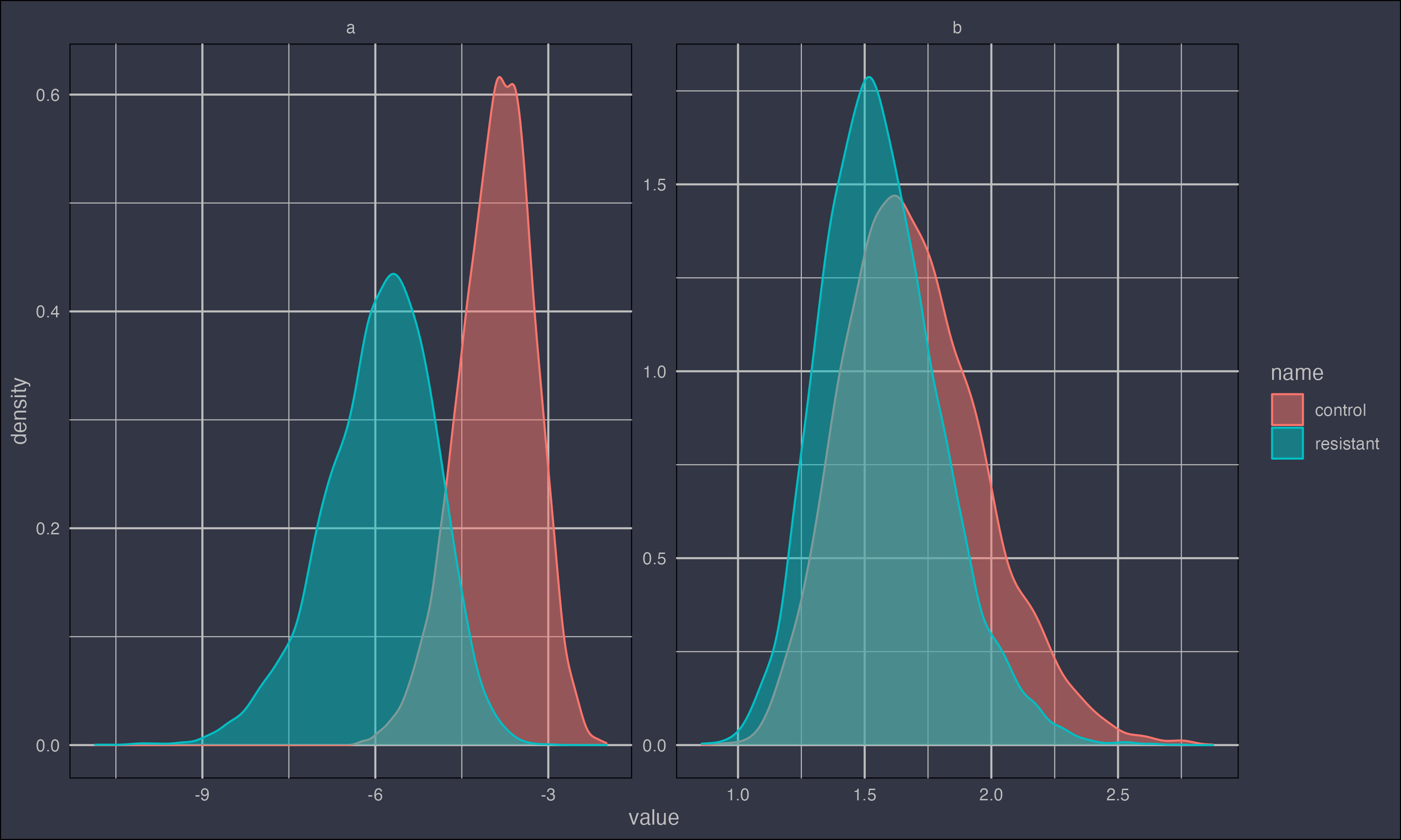
The posterior distribution
One of the cool things about Bayesian approaches is that each parameter is assumed to have a probability distribution (rather than an error). What's more, the posterior probability distributions can take a range of forms, i.e., they are not necessarily normally distributed.
e <- rstan::extract(fit)
a <- tibble(control = e$a[, 1], resistant = e$a[, 2]) %>%
    mutate(par = "a", id = 1:n())
b <- tibble(control = e$b[, 1], resistant = e$b[, 2]) %>%
    mutate(par = "b", id = 1:n())

dl <- bind_rows(a, b) %>%
    pivot_longer(-c(par, id))

ggplot(dl, aes(x = value, color = name, fill = name)) +
    geom_density(alpha = 0.5) +
    facet_wrap(~par, scales = "free") +
    mydarktheme
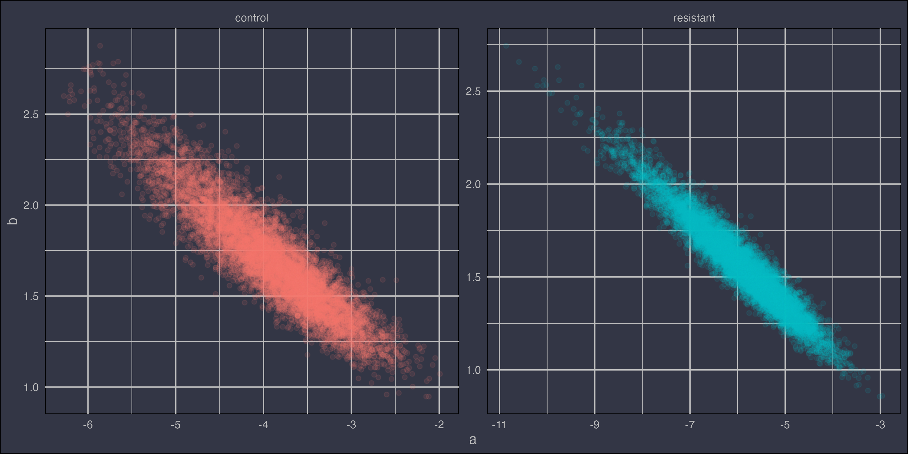
Here we can see how the posterior distributions of the parameters covary with the other parameter estimates. The density of the points corresponds to the probability distribution of the parameters.
dl %>%
    pivot_wider(names_from = par, values_from = value) %>%
    ggplot(aes(a, b, color = name)) +
    geom_point(alpha = 0.1) +
    facet_wrap(~name, scales = "free") +
    mydarktheme +
    guides(color = "none")
Retrieving model predictions from the posterior distribution can be a bit fiddly as there is no analytical expression based on parameter estimates. Rather, parameter samples from the posterior distribution must be transformed into model predictions and the quantiles must be estimated numerically. There are likely packages that can take care of this for you, but I haven't looked into it just yet.
pred <-
    expand.grid(dose = 10^seq(-2, 4, by = 0.1), pop = c(1, 2)) %>%
    as_tibble()

pred$pred <- NA
pred$predu95 <- NA
pred$predl95 <- NA
for (i in 1:nrow(pred)) {
    pop <- pred$pop[i]
    dose <- pred$dose[i]
    logit <- e$a[, pop] + e$b[, pop] * log(dose)
    p <- 1 / (1 + exp(-logit))
    qs <- quantile(p, c(0.025, 0.5, 0.975))
    pred$predl95[i] <- qs[1]
    pred$pred[i] <- qs[2]
    pred$predu95[i] <- qs[3]
}

pred %>%
    mutate(pop = c("control", "resistant")[pop]) %>%
    ggplot(aes(x = dose, y = pred, color = pop, fill = pop)) +
    geom_point(data = d, aes(dose, dead / total, color = pop)) +
    geom_line() +
    geom_ribbon(aes(ymin = predl95, ymax = predu95), alpha = 0.5) +
    mydarktheme +
    xlab("omethoate (mg/L)") +
    ggtitle("Bayesian") +
    scale_x_log10()
Comparing the two model predictions
Hover your mouse over the plot below to compare the two predictions.

